Next: Phase-Transitions and Computation
Up: Computation, Dynamics and the
Previous: Theory of Computation
Subsections
Our discussion of finite automata outlined the workings of a class of simple
machines. Though we did not study their behavior, when given carefully selected
transition functions and placed into particular nested configurations, these
simple machines can exhibit the full range of dynamical behavior: fixed point,
periodic and even chaotic [4]. Since one of our aims is to look
at whether or not an analog of universal computation exists in dynamical systems
(and if so, what that analog is), we find that finite automata might provide
a simply constructed system ideal for study. In fact, as we shall see, it is
possible to generate a system of finite automata that not only exhibit the full
spectrum of dynamical behaviors but are also already known to support universal
computation!
Imagine a lattice with a finite automaton residing at each lattice site. Each
automaton is designed so that its current state is visible to its own input
sensor and the input sensor of the surrounding automata. Each automaton shall
take as input the state configuration displayed by its local neighborhood.
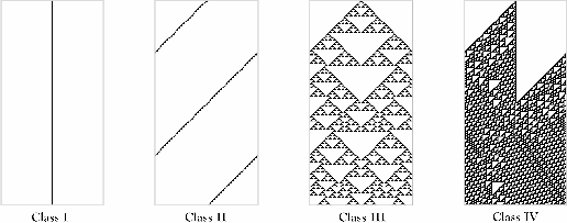
Typically, a CA neighborhood is defined as an automaton and its immediate neighbors.
The two most common neighborhood templates used for a two-dimensional lattice
are:
Figure:
Two most common 2-D CA neighborhood templates.
|
|
Since the automata are using state configurations of a given template as their
input source, the set of all possible configurations for a given template is
isomorphic to the set of input symbols that the automata need recognize.
To simplify construction of CA systems, the following conventions are universally
employed:
- All FA are defined to use the same set of state symbols
 .
.
- All FA use the same neighborhood template
 .
.
- As a consequence of 1 and 2, all FA will be recognizing the exact same set of
state configurations. Thus, it its natural to define all automata to use the
same input symbol alphabet
 .
.
Typically, an FA's accepting states is ignored since the goal of a cellular
automaton is not to accept or reject an input set, but to process an initial
configuration of start states. This leaves the last, arguably most important,
ingredient in a CA, the transition function.
Traditionally, the transition function is defined identically for all FA. This
effectively makes all FA in a cellular automaton duplicates of an archetype
FA. This criteria is known as uniformity. Most of the research and applications
involving CA have been with uniform CA. Recently, some interest has shifted
to non-uniform CAs since it has been shown that they can solve problems that
uniform CAs can not [10].
Time is spent simplifying the CA for study because a cellular automaton having
as few parameters as necessary allows for a high-level search for behavior indicative
of computational ability.
Summary 1
Our current system places a finite automaton at each site in a

-dimensional
lattice. All automata have an identical set of states, use the same neighborhood
template, recognize an identical set of input symbols and behave using the same
transition function.
A valid concern might be that the system created thus far is too limited. Limited,
possibly, to the extent that universal computation may in fact be impossible.
However, the cellular automaton model constructed thus far is the same as that
used in Conway's ``Game of Life''2. That the Game of Life has been proved to be capable of universal computation
is our insurance that such a limited system is not too limited.
Note 1
The Game of Life is one particular choice of transition function for a two-dimensional,
binary-state, uniform cellular automata using the 9-neighborhood template. The
Game of Life has been proved to be universal.
We calculate the total number of rules (transition functions) that are available
to a cellular automata system:
For any neighborhood template, , there are
 cells.
Each contains a finite automaton of
cells.
Each contains a finite automaton of
 -states. Thus, there
are
-states. Thus, there
are
 possible
state configurations. By Proposition
possible
state configurations. By Proposition ![[*]](/usr/share/latex2html/icons/crossref.png) , the total number of
possible rules is
, the total number of
possible rules is
We record this as
Proposition 3
For any uniform system of cellular automata using
the FA
and having a neighborhood template
, there are

rule sets to choose from.
Example
The Game of Life is one particular rule choice for two-dimensional, binary-state,
uniform cellular automata using the 9-neighborhood template. What is the total
number of rules available in this system?
Even though we have attempted to generate for ourselves a CA system of few parameters,
the previous proposition shows us that the size of rule space grows at a phenomenal
rate with the number of states and template size being used. Even if we were
content to study just a single system, we are left with a large, undifferentiated
space of CA rules [6,7].
Our initial goal should then be to impose a structure on the space of rules
that generates a nice ordering on which we could apply an index (a parameterization).
The most ideal structure would partition the space of CA rules into regions
correlated with the various dynamical behaviors observable in CA. By then probing
the regions that exhibit computational abilities, we can begin to draw connections
between the ability for computation and associated dynamical behaviors
We introduce the parameterization employed by Dr. Christopher Langton during
his artificial life explorations of CA space [8].
Definition 2
The  parameter.
 For a uniform,
-state
CA using neighborhood template
and FA
,
let

be known as the
quiescent state and let

contain

transitions to

. Let the remaining

transitions in
be filled by picking randomly and uniformly over
the set of states

. Then we say
To get an idea of how the parameter correlates with the generated
rule set, note the following particular values for :
 |
All transitions in are to the quiescent state . |
 |
No transitions in are to the quiescent state . |
 |
All states are equally represented. |
We use the parameter precisely because it is deficient with
respect to surveying the finer structure of CA space. This blurs the space we
must search in, allowing us a low resolution survey in which we can identify
the interesting areas for future, sharper exploration.3
That
represents the most homogeneous rule sets and
represents the most heterogenous rule sets gives some indication that
is providing the structure we need to effectively search CA space. In fact,
since these values represent end points in the spectrum of rule choice, we shall
restrict our search of CA space to those rules having values
lying within this range.
Searching rule space is the process of stepping through the range
 in discrete steps, and, at each sampled point, characterizing the CA behavior
resulting for , the rule set randomly generated with respect to
. The goal of this process is to describe the relation between
value and CA behavior. From these results comes the ability
to focus in on values displaying interesting dynamical behavior
and possibly harboring computational ability.
in discrete steps, and, at each sampled point, characterizing the CA behavior
resulting for , the rule set randomly generated with respect to
. The goal of this process is to describe the relation between
value and CA behavior. From these results comes the ability
to focus in on values displaying interesting dynamical behavior
and possibly harboring computational ability.
In order to make the studies of CA more tractable, there are a couple of further
restrictions that are commonly placed on how should be defined.
Definition 3
Quiescence restriction. Any neighborhood that is uniform in
cell-state
, the quiescent state, should map to
.
A stronger form of this restriction is known as
Definition 4
Strong quiescence. A neighborhood uniform in any state,

,
should map to

.
Almost universally observed in CA research is the restriction known as
Definition 5
Spatial isotropy. All planar rotations of a neighborhood-state will map
to the same state.
This has the effect that the local dynamics is unable to make use of the global
property of orientation [6].
A Relationship with Dynamical Systems
The study of dynamical systems involves the analysis of phase space.
Phase space is the space of all possible values that a system's variables can
take on. Each point in phase space represents particular values for all of the
system's variables and we refer to this point as the system's state.
A system's phase space (state space) covers all of the states in which
a system could possibly be in.[1]
Example
A thermometer has a one-dimensional state space which can be mathematically
idealized as the real number line. Each point on this line represents a particular
state that the thermometer could be in corresponding with measured temperature.
Note that this particular state space would have a practical lower bound at
the point marking absolute zero.
Example
Relative to the center of Earth, every body has a 6-dimensional state space
which can be represented by a 6 dimensional real vector space. Each point in
this vector space represents a particular state that the body could be in corresponding
with its position and velocity relative to the center of Earth. Three axes could
be devoted to position,

, and three devoted to velocity,

.
As a system changes over time its variables change value. As variables change
value, the state point forms a trajectory path in state space. Dynamical systems
theory has been interested in generalizing system behavior through studying
the geometry of the long term trajectories. Discovered is that there are three
distinct behaviors any system may evolve into:
- fixed point attractive: Behavior stabilizes to a single point in phase
space that is unchanging over time. In general, there is a clear correspondence
between system start state and long term behavior; similar start states producing
similar state path trajectories.
- periodic attractive: Behavior stabilizes into a closed path. In general,
there is a clear correspondence between system start state and long term behavior;
similar start states producing similar state path trajectories.
- chaotic attractive: Behavior never seems to stabilize, however the subspace
in which the state path trajectory moves is restricted to a bounded manifold.
This manifold often possesses complex, detailed structure. In general, similar
start states do not produce similar state path trajectories. This last property
is called sensitivity to initial conditions.
We say that the behavior is attractive because we take the view that there is
some sort of attractor, or potential force, towards which the
state path is evolving.
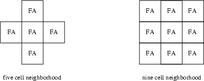
Example 1
A thermometer, initially at room temperature, is heated. Over time, the thermometer
cools down to room temperature again. In phase space, this cooling process would
appear as a point on the real number line sliding towards the value representing
room temperature. We say that the state path trajectory is being attracted to
the point representing room temperature. What would the attractor look like?
Fixed point attractive systems are attracted to a fixed point attractor,
periodic attractive systems are attracted to a periodic attractor and
chaotic attractive systems are attracted to a strange attractor. (See
Figure4 ).
Figure:
Three classes of attractor.
|
|
We are interested in studying how the behavior of cellular automata correlates
with the choice of rule set and whether or not there is a sub-rule-space that
lends itself to computational ability.
The obvious analogue for studying a dynamical system phase space is studying
a cellular automata state space. We described the state of a dynamical system
as the point in phase space representing the current values for all of its variables.
In a similar manner, we can describe the global state of a CA by its current
total configuration of cell states. This makes the CA phase space the set of
all possible global configurations. Thus, the time evolution of a CA could be
studied by observing the state-path trajectory in this set of global configurations.
The natural question following the this analogy is: What kinds of dynamical
behavior do cellular automata exhibit?
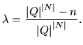
In 1984, Stephen Wolfram undertook a detailed study of one-dimensional cellular
automata and their relationship to dynamical systems [13].
His study identified four distinct classes of cellular automaton behavior (see
Figure5 ):
- Class I
- From almost any initial configuration, cellular automata evolve to
a homogeneous state after a finite number of time steps. Cellular automata in
this class exhibit the maximal possible order on both global and local scales.
- Class II
- Cellular automata usually evolve to short period structures. Local
and global order is exhibited, although not maximal.
- Class III
- Evolution of cellular automata from almost all possible initial states
leads to aperiodic patterns. After sufficiently many time steps, the statistical
properties of these patterns are typically the same for almost all initial configurations.
Cellular automata in this class can exhibit maximal disorder on both
global and local scales.
- Class IV
- Yields stable, periodic and propagating structures which can persist
over arbitrary lengths of time. By properly arranging the propagating structures,
final states with any cycle length may be obtained. The cellular automata in
this class exhibit a great deal of local order.
Figure:
Wolfram class examples. Each image a time-evolution of a 2-state CA on a circle
using neighborhood size of 3 (central cell and its two neighbors).
|
|
For each CA class, Wolfram described the behavior in terms of dynamical systems
theory:
- [Class I]Cellular automata evolve to limit points.
- [Class II]Cellular automata evolve to limit cycles.
- [Class III]Cellular automata evolve to strange attractors.
- [Class IV]Cellular automata exhibit very long transient lengths, having no direct
analogue in the field of dynamical systems.
One way of probing a system's behavior is to put it into a state of non-typical
behavior and watch the resulting behavior as the system moves towards its attractor.
This interim behavior, between perturbed and settled behavior, is known as the
transient behavior. Of interest is how the transient times change with
regard to the size of the system under study.
For fixed-point and periodic systems, the effects of perturbations are restricted
within a finite region of the FA array. In other words, beyond this region,
the other cells in the array feel neither direct nor indirect effects of the
perturbation. These finite regions are typically small and independent of the
array size. The relation between the size of a cellular automaton and the average
length of its transients is summarized:
- fixed-point systems
- Transient length is independent of system size.
- periodic systems
- Transient length is dependent on system size taking on a number
of different forms related to how long it takes for localized regions to settle.
- chaotic systems
- Perturbations are quickly randomized, making their effect on
local regions independent of system size. This would be akin to throwing a rock
into a pond during a rain storm.
For systems in between, transients show a dependence on system size taking on
a variety of functional forms. It is also possible for transients in this dynamical
system regime to become effectively infinite -- the system spends virtually
all its time on a transient.
``Cellular automata can be viewed either as computers themselves or as logical
universes, within which computers may be embedded.''6
As ``computers themselves'', cellular automata use their starting configuration
as the data which their transition function is to process. This means the function
is representing the algorithm being computed for the input data.
As ``logical universes within which computers may be embedded'', a cellular
automaton's starting configuration constitutes a computer with input data and
algorithm. Suitable initial configurations can specify arbitrary algorithmic
procedures and input data, thus the system serves as a general purpose computer.
In this scenario, the CA transition function is acting as the ``physics''
under which this general purpose computer will operate.
The Game of Life is a concrete example that CA can support universal computation.
However, that CA can be functionally universal has been known since their invention
by Ulam and von Neumann in the 1940s. Von Neumann invented cellular automata
because he was searching for a mechanism by which machines could self-reproduce.
In his existence proof of such self-reproducing machines, von Neumann demonstrated
the existence of a universal computer using a two-dimensional, 29-state cellular
automaton with the 5-neighborhood template. From this proof stemmed subsequent
proofs of automata with much fewer states supporting universal computation.
The technique for showing a system universal general involves constructing the
necessary and sufficient parts of a computer inside of that proposed system.
Some of these proofs involve the construction of Turing machines, other involve
the construction of the more modern notion of a stored-program computer. An
example of this latter technique was recently given when the spatialized prisoner's
dilemma was shown to be universal. An appropriate choice for dilemma payoff
matrix allows for the construction of a virtual Minsky register machine [5].
A Minsky register machine is a general purpose electronic computer.
What sort of factors or criteria are needed for a system to be capable of universal
computation? It is the dynamics of the transition function ``physics'' that
provides the conditions for these constructive proofs of universality. In particular,
three fundamental features have been determined as necessary and sufficient
for these constructions:
- The dynamics must support the storage of information. This entails the
ability for local regions of state information to be preserved for arbitrarily
long times.
- The dynamics must support the transmission of information. This entails
the ability for small (local) regions of state information to propagate over
arbitrarily long distances.
- Stored and transmitted information must be able to interact, resulting in a
possible modification of one or the other.
Taken together, we see that a dynamical system must be able to correlate storage
and transmission abilities (condition 3) and that this correlation can be arbitrarily
long (conditions 1 & 2). Like a Turing machine tape, these correlation lengths
should be finite, but unbounded.
In his development of the CA classification, Wolfram suggested that Class IV
CA are capable of supporting computation, noting similarities between structures
observed in his studies and the Game of Life [13].
Langton theorized that it is the association between Class IV CA and very long
transients that explains their computational capacity and the difficulty to
characterize their behavior.
A Search of CA Space
We give a description of one of Langton's [6,7] explorations
of CA space via the parameter.
The search took place on a one-dimensional lattice having 128 sites wrapped
into a circle. Thus, the time evolution of this system would be best displayed
on a cylinder; each additional time-step being, conventionally, placed below
the last. The lattice is uniform with 4-state FAs using a neighborhood of size
5 (the central cell, two cells on its left and two cells on its right). Each
CA was initialized in on of two ways:
- A uniform, random configuration of initial states is given to all 128 cells.
- On a quiescent background, a uniform, random configuration of non-quiescent
initial states is given to the center 20 cells.
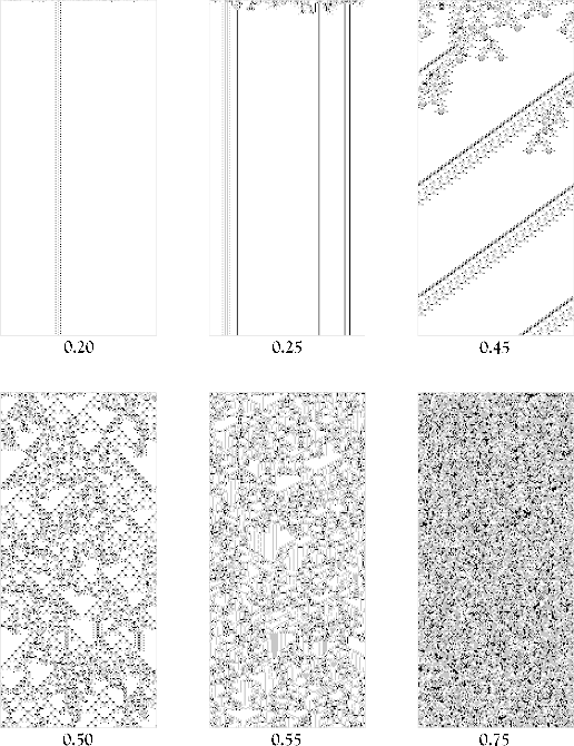
The search produced the following primary dynamical features (see Figure7 ):
Figure:
For selected
-values, a 256 step time-evolution
of a corresponding CA.
|
|
- [
 ]After a single time-step, the array is uniform
in . Systems are characterizable as immediately decaying to a fixed-point
attractor.
]After a single time-step, the array is uniform
in . Systems are characterizable as immediately decaying to a fixed-point
attractor.
- [
 ]Decay to uniformity in takes between
4 or 5 time-steps. We refer to this activity as the transients, since
it precedes the ``typical'', long-term behavior.
]Decay to uniformity in takes between
4 or 5 time-steps. We refer to this activity as the transients, since
it precedes the ``typical'', long-term behavior.
- [
 ]Systems can now also produce potentially permanent
periodic structures. Transient length is between 7 and 10 time-steps.
]Systems can now also produce potentially permanent
periodic structures. Transient length is between 7 and 10 time-steps.
- [
 ]Systems can now also produce cells that get stuck
in a single, non-quiescent state. Langton referred to these as period 1 structures.
]Systems can now also produce cells that get stuck
in a single, non-quiescent state. Langton referred to these as period 1 structures.
- [
 ]Periodic structures are observed with periods of
up to 40 time-steps. Transient length has increased to 60 time-steps. Globally,
systems can be characterized as collapsing into isolated areas of periodic activity.
]Periodic structures are observed with periods of
up to 40 time-steps. Transient length has increased to 60 time-steps. Globally,
systems can be characterized as collapsing into isolated areas of periodic activity.
- [
 ]Transient length has gone through a dramatic increase
to almost 1000 time-steps. Globally, systems appear to be near a balance between
collapsing and expanding dynamical activity. Being near this balance seems to
give systems the ability to produce propagating structures. These propagating
structures may appear, on first look, to be period 100 structures. However,
extended observation of the cycling allows one to notice that a whole structure
is slowly gliding around the lattice circle. Thus, the true period length of
this structure includes the time it takes to orbit around the circle until reaching
the initial location and configuration. In Langton's study, the structure under
his observation had to orbit 3 times before repeating exactly. Taking 116 time-steps
to shift 3 sites, the true period of this structure was
]Transient length has gone through a dramatic increase
to almost 1000 time-steps. Globally, systems appear to be near a balance between
collapsing and expanding dynamical activity. Being near this balance seems to
give systems the ability to produce propagating structures. These propagating
structures may appear, on first look, to be period 100 structures. However,
extended observation of the cycling allows one to notice that a whole structure
is slowly gliding around the lattice circle. Thus, the true period length of
this structure includes the time it takes to orbit around the circle until reaching
the initial location and configuration. In Langton's study, the structure under
his observation had to orbit 3 times before repeating exactly. Taking 116 time-steps
to shift 3 sites, the true period of this structure was
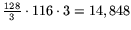 time-steps! Systems generated with respect to this value do
not necessarily produce these propagating structures.
time-steps! Systems generated with respect to this value do
not necessarily produce these propagating structures.
- [
 ]Transient length is dramatically increasing; now
on the order of 12,000 time-steps. It is unclear whether or not the global behavior
is expanding or contracting. Langton hypothesizes an overall expansive nature
that is eventually destroyed by the wild fluctuations of dynamic activity, leaving
periodic structure residue.
]Transient length is dramatically increasing; now
on the order of 12,000 time-steps. It is unclear whether or not the global behavior
is expanding or contracting. Langton hypothesizes an overall expansive nature
that is eventually destroyed by the wild fluctuations of dynamic activity, leaving
periodic structure residue.
- [
 ]Transient activity has become so long that it
can be considered to be the ``typical'', long-term behavior. In this new dynamical
regime, long-term behavior now tends to chaotic behavior.
]Transient activity has become so long that it
can be considered to be the ``typical'', long-term behavior. In this new dynamical
regime, long-term behavior now tends to chaotic behavior.
- [
 ]Transient activity decreases as
increases. Again, this means that the time it takes for the system to reach
is ``typical'', long-term behavior has become increasingly shorter. We say
that a chaotic system has reached its ``typical'', long-term behavior when
the density of occupied lattice sites is within 1% of the long-term average.
When
]Transient activity decreases as
increases. Again, this means that the time it takes for the system to reach
is ``typical'', long-term behavior has become increasingly shorter. We say
that a chaotic system has reached its ``typical'', long-term behavior when
the density of occupied lattice sites is within 1% of the long-term average.
When
 , systems become ``typically'' chaotic after
only a single time step. Compare this to
, systems become ``typically'' chaotic after
only a single time step. Compare this to
 where it
takes approximately 10 time-steps. In other words, systems are characterizable
by very quick decays to a strange attractor.
where it
takes approximately 10 time-steps. In other words, systems are characterizable
by very quick decays to a strange attractor.
By varying the parameter, we are able progress through CAs exhibiting
maximal possible order to CAs exhibiting maximal possible disorder. At either
end of the spectrum, behavior can be characterized as quickly decaying to its
long-term attractor. In the middle of the spectrum, behavior becomes very unpredictable
with long transients preceding a break down to long-term behavior. Also, we
were able to witness a very rapid increase in transient length. This ultimately
led to a new regime of dynamical behavior which had its own transient lengths
very rapidly decrease as increased. This dynamical regime separating
the periodic regime from the chaotic regime is known as the transition
regime.
The transition regime is able to support propagating structures (as discussed
above for
). These structures are very much like
the ``gliders''8 seen in the Game of Life. It is interesting to note, that for CAs using the
parameters of the Game of Life, the value corresponding to the
Game of Life's particular rule choice lies within the transition regime. By
increasing the lattice size for the above experiment, the existence of several
different kinds of propagating structures can be observed. Langton found that
the collision between a propagating structure and a static structure produces
a structure which propagates in the opposite direction. It is exciting to realize
that these interactions can create a basis for transmission, storage and modification
of structurally embedded information. Thus, this transition regime seems to
harbor the ingredients for constructing a universal computer.
Footnotes
- ... Life''2
- The Game of Life is a system well studied for both scientific and
recreational purposes. Many resources exist for learning and exploring
this system. One such resource is
Paul's Page of
Conway's Life Miscellany
http://www.cs.jhu.edu/callahan/lifepage.html
- ... exploration.3
- Chris Langton notes that H. A. Gutowitz has defined a hierarchy of parameterization
schemes in which is the simplest. References are given in his
PhD Thesis [6] and Physica D article [7].
- ...
Figure4
- Fixed-point and periodic attractor images were borrowed from Dynamics:
The geometry of Behavior [1]. Strange attractor was generated
with Theory.org's
*BFE software suite [11].
- ...
Figure5
- Images were generated using the
``elementary CA'' form at
Santa Fe Institute's
Artificial Life OnLine
website [2].
- ... embedded.''6
- Chris Langton, Physica D 42, p. 15. [7]
- ... Figure7
- Images were generated using the
``lambda CA form'' at
Santa Fe Institute's
Artificial Life OnLine
website [2].
- ... ``gliders''8
- Glider Description
http://www.brunel.ac.uk/depts/AI/alife/al-osc.htm#glider
Next: Phase-Transitions and Computation
Up: Computation, Dynamics and the
Previous: Theory of Computation
Jeremy Avnet (brainsik); Senior Thesis, Mathematics; University California, Santa Cruz; 6th June 2000; email: jeremy (at) theory.org