BSpline interpolation

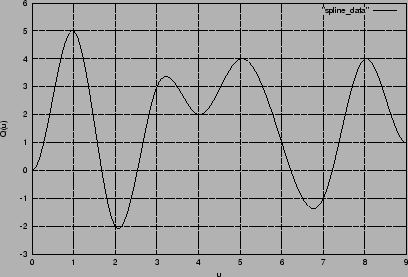
one dimensional spline example

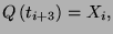
The BSpline interpolation is implemented as described in [watt92]. Input is a set of n one dimensional data points X_i and a knot vector containing n+6 knots. A set of n+2 control points p_i are generated so that a cubic spline with those control points will fit the data. The control points are such that p₀=p₁ and p_n+1=p_n+2. We also subject the curve to the constraint that This means that the curve is defined over the interval This system of equations is then solved to get the control points for the curve.

The curve at time u is given by a weighted sum of the control points 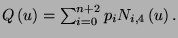The Blending functions are as follows:

$$N_{i,1}\left( u\right) =\left\{ \begin{array}{ll} 1 & \textr... ...{i}\leq u<t_{i+1}\\ 0 & \textrm{otherwise} \end{array}\right.$$

$$N_{i,k}\left( u\right) =\frac{\left( u-t_{i}\right) N_{i,k-1... ... t_{i+k}-u\right) N_{i+1,k+1}\left( u\right) }{t_{i+k}-t_{i+1}}$$

Higher dimensional interpolants can be generated by interpolating each element independently.

In general, the interpolation of a parameter proceeds as follows:

 

control_points = get_control_points(data, knots);

 

interpolant = spline_at(t, control_points);