Introduction to the Theory of Cellular Automata and
One-Dimensional Traffic Simulation
Richard Cochinos
Abstract
This paper is roughly divided into two parts. After a brief
introduction, I will discuss the theory and properties underlying
cellular automata. Included in this section will be a definition, a
list of the physical properties, rules and rules assigning, and a
description of some of the dynamical properties inherent in
automata. The second section of this paper will be devoted to
discussing cellular automata as a model for traffic flow. It will
include a one-dimensional example and conclusions from the
model.
Background
I became interested in cellular automata after engaging in a
project to model human behavior. My idea for an art installation was
to fill a gallery volume with twenty 8’ high columns, placed
far enough apart so you could easily walk through them. The sides of
the columns were to be painted various colors, with only one
entrance/exit into the space. The question I was engaged with at the
time was how would people react and interact with color when you
present them with multiple distinct decisions. For the duration of
the show I would record movement with a video camera placed on the
ceiling. I was hoping to discover inherent patterns of movement
across the floor, from various repellors to various attractors. I
was then going to use what is known about color psychology to arrive
at(if any) conclusions. The installation was never built due to the
cost of the project and the time involved in construction. However,
I decided to take the concept as far as I could intellectually. This
led me to the problem of accurately describing the dynamics of
people interacting with each other and objects within a finite
space. I was then introduced to cellular automata as a modeling
system. This paper is a continuation of that study.
Introduction
The basis of my decision to examine cellular automata (CA) as a
model for traffic was its logical parallelism to modeling human
behavior through closed spaces. More and more metropolitan areas
suffer from an increased transportation demand which largely exceeds
capacity. In many cases it is not possible, or even desirable, to
extend capacity to meet the demand. In consequence, the consistent
management of large, distributed man-made transportation systems has
become more and more important. However, until these are in place a
reliable transportation system must exist. A first step in
‘reliability’ is understanding how these systems behave.
CA’s are an alternative to Differential Equations in an attempt
to model these systems. CA models have the desirable capacity to
capture micro-level dynamics and relate these to macro-level
behavior. Cellular Automata models are capable of representing
individual vehicle interactions and relating these interactions to
macroscopic traffic flow metrics, such as throughput, time travel
and vehicle speed. By allowing different vehicles to possess
different driving behaviors CA models can adequately capture the
complexity of traffic.
This paper will mainly discuss the theory behind cellular
automata. It is expansive, so not everything could be included.
Before concluding I will work through a 1-dimentional traffic model
as an example of several of the outlined concepts.
Definition
Because of CA’s utility in so many disciplines, there are
multiple ways in which an automaton can be defined. For our purposes
I have concentrated on the physical and mathematical aspects which
are necessary for understanding traffic simulation. The following
are two universal definitions given by Lyman Hurd from Georgia
Tech.:
Physicists View:
A cellular automaton is a discrete dynamical system. Each point in
a regular spatial lattice, called a cell, can have any one of a
finite number of states. The states in the cells of a lattice are
updated according to a local rule. That is, the state of the cell
at a given time depends only on its own state one time step
previously, and the states of its nearby neighbors at the previous
time step. All cells in the lattice are updated synchronously. The
state of the lattice advances in discrete time steps.
Mathematicians View:
Notation: d=dimension
k=states per site
r=radius
For simplicity, assume d=1 for the moment.
A d-dimensional cellular automaton takes as its underlying space
the lattice (integers) where S is a finite set of k elements. The
dynamics are determined by a global function

whose dynamics are determined ``locally'' as defined below. A
``local (or neighborhood) function'' f is defined on a finite
region

The all-important property of cellular automata, is that this
function is defined discretely (a finite lookup table). Both the
domain and range of f are finite. The global function F arises
from f by defining:

(hurd@gatech.edu)
Some relevant facts from a topological standpoint are:
1. The base space is compact and the global function F is continuous.
2. The map F commutes with the shift operator which takes Ci to Ci+1.
In fact, cellular automata are characterized completely by
properties 1 and 2 . According to Hurd, this makes CA are an ideal
meeting point between continuous dynamics and complexity theory,
since they are discretely defined but exhibit continuous dynamics.
The transition to more dimensions is straightforward. The only
difference is that the global function F is defined over S
(functions from a d-dimensional lattice to S) and the local function
f is determined by enumerating the image of all patches of size 2
(Gutowitz)
Physical Properties
Because automata are not solely mathematics but modeling systems,
it is helpful to understand the
physical properties of the automata. These can be divided into three
parts, the cell and lattice, the neighborhood, and the rules.
The basic element of an automata is the cell. The cell is a
memory element and stores states. In the simplest case each cell can
have the binary states 1 or 0, or a finite amount of states in
complex simulations. These cells are arranged in a spatial web -- a
lattice. The simplest one being the one-dimensional lattice, meaning
that all the cells are arranged in a line like a string of pearls.
The most common CA’s are built in one or two dimensions, for
computational limits. Because there is a much smaller possible set
of 'rules', which will be discussed later, 1-D CA’s have been
explored more by theoreticians.
Up to now these cells arranged in a lattice represent a static
state. To introduce dynamic into the system, we have to add rules.
The 'job' of these rules is to define the state of the cell for the
next time in dependence of the neighborhood cells. Different
definitions of neighborhoods are possible, each one being more or
less effective depending on the system you wish to model. Concerning
the two dimensional lattice the following definitions are
common:
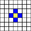
von Neumann Neighborhood
four cells, the cell above and below, right and left from each cell
are called the von Neumann neighborhood of this cell. The radius of
this definition is 1, as only the next layer is considered.
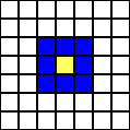
Moore Neighborhood
the Moore neighborhood is an enlargement of the von Neumann
neighborhood containing the diagonal cells too. In this case, the
radius r=1 too.
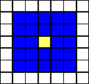
Extended Moore Neighborhood
equivalent to description of Moore neighborhood above, but
neighborhood reaches over the distance of the next adjacent cells.
Hence the r=2 (or larger).
Margolus Neighborhood
a completely different approach: considers 2x2 cells of a lattice at
once.


von Neumann Neighborhood Moore Neighborhood Extended Moore Neighborhood
The blue cells are the neighborhood cells to the center (core)
cell. As discussed before the states of these cells are used to
calculate the next state of the center cell according to the defined
rule. As the number the number of cells in a lattice has to be
finite, one problem occurs considering the neighborhoods described
above: What to do with cells at the borders? The influence depends
on the size of the lattice. To give an example: In a 10x10 lattice
about 40% of the cells are border cells, in a 100x100 lattice only
about 4% of the cells are of that kind. Regardless, this problem
must be solved. Two solutions are common:
1.Opposite borders of the lattice are "stuck together". A one-dimensional "line" becomes
a circle, a two dimensional lattice becomes a torus.
2. The border cells are mirrored: the consequence is symmetric border properties.
The more usual method chosen is (1) however, border definitions are
infinite (Schatten).
Rule Evolution of the CA
Evolutionary properties of the automata are properties that are
affected by a rule. A nice example rule evolution is 'the wave' in a
sports stadium. Each person reacts only to the state of his
neighbor(s). If they stand up, (s)he will stand up too, and after a
short while, (s)he sits down again. This illustrates the most
important concept for automata: Local interaction leads to global
dynamic. This dynamic is governed by rules. Interestingly all rules
can be arranged into three classes:
1. Every group of states of the neighborhood cells is
related a state of the core cell. E.g.
consider a one-dimensional CA: a rule could be "011 ->
x0x", what means that the core cell
becomes a 0 in the next time step (generation) if the left cell is
0, the right cell is 1 and the core cell is 1. Every possible
state has to be described.
2. "Totalistic" Rules: the state of the next state core cell is only dependent upon the sum of
the states of the neighborhood cells. E.g. if the sum of the
adjacent cells is 4 the state of the
core cell is 1, in all other cases the state of the core cell is 0.
3. "Legal" Rules: a special kind of totalistic
rules are the legal rules. As it is not of
advantage in most cases to use rules that produce a pattern from
total zero-state lattices (all
cells in the automaton are 0), Wolfram defined the so called legal
rules as a subset of all possible rules, a selection of rules that
produce no ones from zero-state lattices (Schatten).
Rule 1 shows why one-dimensional automata are most popular in
theoretical studies. If only the left, the right neighbor and the
cell itself are considered(r=1), there are 256 possible rules. 2 =8
possible states for three binary digits. Each of these 8 states can
produce a 1 or a 0 for the center cell in the next generation. Hence
2 =256 rules are existing. In general, the number of rules can be
calculated by , where k is the number of states for the cell and n
is the number of neighbors. We can easily see for a two-dimensional
automata with a Moore neighborhood and 2 states, it follows k=2 and
n=9. So =262,144 possible rules exist. A comprehensive study of all
rules in higher dimensional automata is thus not easily possible
(Schatten).
Rule Assigning
Rules may be generalized in various ways. One family of rules is
obtained by allowing the value of a site to be an arbitrary function
of the values of the site itself and two of its nearest neighbors on
the previous time step(rule class 1).

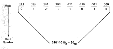
It is possible to assign a convenient notation called ‘rule
numbers’. Remember there are 256 rules of this type. Let us
define the rule :
a(i)t+1=a(i-1)t+a(i+1)t mod 2 (1)
The figure below illustrates the conversion of all possible
rule outcomes in binary code to hexadecimal code. Rule (1) is
assigned the rule number 90 in this notation. As a note, rule
numbers are not limited to functions of this type.

As stated before, the number of different rules, with given k
and n, grows by . The only problem is that for relatively small
values of k and n the number of rules is immense. The figure below
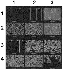
shows examples of evolution according to different rules with
various k and r values

(Wolfram 420)
Each separate rule leads to patterns that differ in detail,
however the examples suggest a remarkable result: all patterns
appear to fall into only four qualitative classes. Wolfram
characterized these basic classes of behavior into:
- Class 1 – evolution tends to a homogeneous state (limiting points) in which, for example, all sites have value 0 – row 1 column 1, (1,1)
- Class 2 – evolution leads to a set of stable or periodic structures (limiting cycle), that are separate and simple - (1,2),(1,3),(3,1)
- Class 3 – evolution leads to a chaotic pattern or ‘strange attractor’– all remainder images except (4,3)
- Class 4 – evolution leads to complex structures, sometimes long-lived - image (4,3)
The existence of only 4 classes implies universality in the behavior of CA. The implications of this are large enough to extend beyond the scope of this paper. What is interesting though an adequate explanation has yet to be conjected.
Properties of CA
Before moving on, I think it important to summarize the physical and evolutionary properties of cellular automata:
- CA´s develop in space and time
- a CA is a discrete simulation method, hence Space and Time are defined in discrete steps.
- a CA is built up from cells, that are lined up in a string for one-dimensional automata
arranged in a two or higher dimensional lattice for two- or higher dimensional automata
- the number of states of each cell is finite
- the states of each cell are discrete
- all cells are identical
- the future state of each cell depends only of the current state of the cell and the states of the cells in the neighborhood
- the development of each cell is defined by rules
- rules fall into three basic classes
- evolution of these rules leads to dynamical patterns that fall into four classes
Dynamical properties
As CA simulations evolve ‘dynamical’ properties arise. Basically these are patterns we see again and again in varying models. Let us consider 1-D CA sites with the value of 0 or 1. Take the value of position i at time t to be a(i)t . For continuity we will use the same rule as before:
According to this rule, the value of a particular site is given
by the sum modulo 2 of the values of
its left and right nearest neighbor sites on the previous time step,
therefore, it is a totalistic rule.


figure 1figure 2
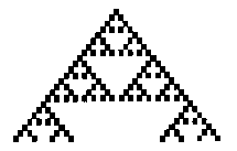
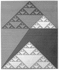
Figure 1 is an image of the evolution generated by eq (1) from a
single seed after 23 time steps, figure 2 shows the pattern
generated after 500 time steps. These are exemplifying
'self-similarity'. As illustrated, portions of the pattern when
magnified are indistinguishable from the whole. Differences on a
small scale between the original pattern and the magnified portion
disappear when one considers the limiting pattern obtained after
an infinite number of time steps. The pattern is therefore
invariant under resealing of lengths. Such a self-similar pattern
is often called a fractal and is characterized by a fractal
diminution.

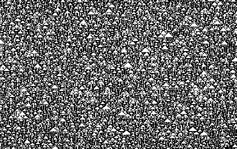
The image above shows the evolution of equation 1 from a
disordered initial state. The values of sites in the initial state
are randomly chosen: each site taking on the value 0 or 1 with
equal probability, independent of the values of other sites. Even
though the initial state has no structure, evolution of the
automata manifests some composition in the form of triangle
‘clearings’. The spontaneous appearance of these
clearings is a simple example of ‘self-organization’.
Both ‘self-similarity’ and ‘self-organization’
are well characterized collective phenomena, seen often in
dynamical fields. The following two properties are intimately
related governing how models are studied. These models are
reversibility and irreversibility.
Irreversibility
A notable feature in the image atop is that the trajectories
merge with time. The merging of trajectories implies that
information is lost in the evolution of the cellular automaton; the
evolution is irreversible. The irreversible evolution decreases the
possibility of some configurations and increases those for others.
The possibility of self organization is therefore a consequence of
irreversibility and the structures obtained through
self-organization are determined by the characteristics of the
attractors. This is an important concept in the fact that most
natural systems exhibit irreversible trends in their evolution. CA
models can mimic this behavior unlike statistical mechanics which
exhibits reversible properties. While there is every evidence that
the fundamental laws of physics are reversible, many systems behave
irreversibly on a macroscopic scale and are appropriately described
by irreversible laws. Cellular Automata provide mathematical models
at this macroscopic level.
Reversibility
The "only" difference to the CA´s described above
is, that the time development of the system is completely
reversible. That means, that at any time-step of the development,
the rules allow to go forward or back in time without losing any
information. Naturally most systems exhibit irreversible behavior,
however constructed dynamical systems, such as traffic, usually
counter this trend.
Now that we have briefly glazed over the important points in CA
theory, we now move on to the construction and description of a
concrete 1-D automaton traffic model.
Traffic Flow models in literature
Traffic flow models can be divided into two major categories:
microscopic and macroscopic. Microscopic models describe behavior as
emerging from discrete entities interacting with each other.
Macroscopic models are concerned with describing aggregate behavior
by characterizing the fundamental relationships between vehicle
speed, flow, and density (Benjaafar 3).
A major limitation of existing microscopic models is that they
assume uniform behavior for all vehicles (ibid, 3). The models are
deterministic, and therefore cannot capture inherent variation in
real traffic vehicle behavior. Microscopic models are also difficult
to extend to multi-lane systems. A key limitation of macroscopic
simulation is their aggregate nature. Because they treat traffic
flow as continuous, they are incapable of capturing the discrete
dynamics which arise from the interactions of individual vehicles.
For example, modeling different behaviors with regard to
acceleration/deceleration or lane changing is difficult. In
addition, because they are deterministic, these models can provide
only average traffic flow metrics. Higher moments of throughput,
travel time, and speed are impossible to characterize. The
usefulness of most of these models is limited to characterizing the
long run behavior of traffic flow and cannot be used for real time
traffic analysis and control (ibid 3).
Cellular Automata for one lane traffic flow
Our initial traffic model is defined as a one-dimensional array
with L cells with closed (periodic) boundaries. This means the total
number of vehicles N in the system is maintained constant. Each cell
may be occupied by one vehicle or it may be empty. Each cell
corresponds to a road segment with length l. Traffic density is the
given by µ=N/L. Each velocity can have a velocity from 0 to
vmax. The velocity corresponds to the number of sites that a vehicle
advances in one iteration. The movement of vehicles throughout the
cells is determined by a set of updating rules. These rules are
applied in a parallel fashion to each vehicle at each iteration. The
length of an iteration can be chosen to reflect the desired level of
simulation detail. The choice of a sufficiently small iteration can
thus be used to approximate a continuous time system. The state of a
system at an iteration is determined by the distribution of vehicles
among the cells and the speed of each vehicle in each cell. We adopt
the following notation:
x(i): position of the ith vehicle
v(i): speed of the ith vehicle
g(i): gap between the ith and the (i+1)th vehicle, given by g(i)=x(i+1) - x(i) – 1
For our model we adapt the following set of rules:
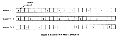
1) Acceleration of free vehicles: If v(i)<vmax and g(i)>v(i)+1, then v(i+1)=v(i)+1
2) Slowing down due to other vehicles: If v(i)>g(i)-1, then v(i)=g(i)
3) Vehicle Motion: Vehicle is advanced v(i) sites
Figure 1 shows the application of these three updating rules to an example system with 24 cells and 7 vehicles:

Under these rules all vehicles have identical behavior and obey the same maximum speed, 5.
Benjaafar, Dooley and Setyawan, three graduate students at
University of Minnesota, based a study on such a model. They were
able to show that speed variance of the individual vehicles
increased dramatically as the system approached maximum flow, the
goal of most traffic plans. Often metro centers attempt to push
roadways to maximum flow since they believe they are getting more
cars through in the same finite amount of time. High speed variance
means that different vehicles in the system have widely varying
speeds. It also means that a vehicle would experience frequent speed
changes per trip through the system. In turn, this results greater
variability in the travel time. In reality, this increases the
possibility of traffic accidents. Thus, it would seem reasonable to
steer traffic away from the density of maximum flow, a
recommendation counter to prevailing practice (Benjafarr 7).
Because we are using a deterministic, reversible and finite CA
model with periodic boundaries, the corresponding traffic system is
periodic in its system states. That is, the number of iterations
necessary to bring back the same state is always finite. Again,
Benjaafar et. al. were able to show that small changes in density
could relate in large fluctuations in this period length. When
applied to a ‘real’ situation, a car that immediately
slows 5 mph during rush hour will have a significant impact on all
those traveling behind it. This influence will take longer to
dispense because of the density that time of day. In practice, a
traffic system with a small period length is more desirable, being
that system is easier to predict and control (Benjaafar 5). Although
these examples are very intuitive more complex models show more
complex behavior. It is not within the scope of this paper to
discuss such systems.
Before closing I would like to inject that deterministic CA are
useful as a modeling paradigm for automated highway systems, where
vehicle speeding and vehicle deceleration are externally controlled.
Indeed, an automated highway system would operate very much like a
deterministic CA with rules specifying the total number of vehicles
allowed in the system and the set of allowable vehicle
behaviors.
Conclusion
As stated before, CA’s developed as an alternative to
partial differential equations. Like variations on counting systems,
they are neither more or less effective, merely different. One of
the nice feature cellular automata have is their information is not
presented abstractly. Because all of the output of CA’s is in
visual form, the average layman can understand the dynamics the
model represents. In this paper I have attempted to give a brief
overview of the theory behind automata as well as a concrete example
in 1-D CA simulation. As stated in the background, this study began
with the question of modeling human behavior in a finite closed
space. From a programming standpoint, the transition from a one to a
two-dimensional model is not that much more difficult. It is within
the 2-D environment that the traffic modeling system becomes
parallel with my original question. However promising this new
system may seem, it should be stated the CA models are greatly
simplified versions of reality. With advances in technology, newer
computers are capable of more and faster calculations, hence greater
accuracy. Like the notion of limits, these massively parallel
machines are giving us insights into the fundamental behavior and
pattern which surrounds our daily life, not through imitation –
but approximation.
Works Cited:
- Alife Online. Ed. Howard Gutowitz, CA FAQ,
Santa Fe Institute,
April 5 1999,
http://alife.santafe.edu/alife/topics/cas/ca-faq/ca-faq.html
- Benjaafar, Saifallah et al., Cellular Automata for Traffic Flow Modeling, Univ. of Minnesota,
Minneapolis, 1997
- Schatten, Alexander, Cellular Automata Digital Worlds,
http://qspr03.tuwien.ac.at/~aschatt/info/ca/ca.html
- Sipper, Moshe, A Brief introduction to Cellular Automata,
http://lslwww.epfl.ch/~moshes/ca.html
- Wolfram, Stephan, Cellular Automata and Complexity, Addison-Wesley, Menlo Park, 1994
Richard Cochinos; email: richard@theory.org
Sat Jun 17 19:24:12 PDT 2000
![]()
![]()
![]()
